On this page, we explore the concept of conditional coloring. It is an innovative concept in graph theory that expands traditional boundaries by adding a specific mathematical or logical function to each edge.
If you are exploring graph theory for the first time, you might be familiar with the classic concept of "proper graph coloring." The traditional rule is very straightforward: you assign a color (which can represent a state, a frequency, or a label) to each point (called a vertex) in a graph so that no two connected points share the exact same color. While this simple rule is highly useful for basic optimization problems, real-world technological challenges demand much more flexibility.
To solve more complex problems, we propose the definition of conditional coloring in such a way that it fundamentally transforms how the connections (called edges) behave. Instead of applying a single, rigid rule to the entire graph, conditional coloring allows every individual edge to dictate its own specific condition about which colors its connected vertices can take.
Adding Functions to the Edges
In standard graph coloring, the implicit rule—or "function"—on every single edge connecting vertex a and vertex b is always exactly the same:
a ≠ b
Under conditional coloring, we remove this limitation entirely. We establish that an edge can hold any arbitrary mathematical or logical function. For example, the restriction function on a specific edge could be defined as:
a ≠ b + 1
...or absolutely any other custom function you need to define. From this perspective, traditional graph coloring is no longer the absolute rule, but merely a specific, basic case of conditional coloring where every edge happens to share the exact same simple inequality constraint. By upgrading edges to contain customized functions, the graph is transformed into a dynamic constraint network.
Explaining Edge Weights as Functions
This new approach also completely redefines how we understand "weighted graphs." Traditionally, a weight is just a static number added to an edge to represent a physical distance, a cost, or a capacity limit.
Through conditional coloring, we can explain these weights in a completely new way: each edge acts as an independent function. Instead of an edge merely carrying a passive number, it dynamically evaluates the relationship between its connected nodes. The "weight" behaves as an embedded parameter or operation within that edge's unique function, actively determining the valid states (or colors) that the connected vertices are allowed to take.
Explaining Edge Directionality as a Function
Furthermore, this approach provides a seamless way to explain the directionality of an edge. In traditional graph theory, directed graphs (digraphs) rely on structural arrows to indicate a one-way relationship or flow between two vertices.
Through the lens of conditional coloring, directionality does not need to be a separate structural property of the graph. Instead, it can simply be represented as a function. By assigning an asymmetric mathematical or logical function to an edge, we inherently create a directed relationship between the connected vertices.
For example, a symmetric function like a ≠ b leaves the edge effectively undirected because the rule applies equally in both directions (since a ≠ b is exactly the same as b ≠ a). However, if we apply an asymmetric restriction such as b = a + 1, we are explicitly treating one vertex as the input and the other as the output. The function itself enforces a strict, one-way mathematical flow.
In this way, the direction of an edge becomes a natural byproduct of the logic assigned to it. This elegantly unifies both directed and undirected graphs under a single, cohesive framework, where the arrow of a directed edge is just another condition embedded within the edge's unique function.
Why is Conditional Coloring Useful?
By replacing rigid structural rules with flexible, edge-specific mathematical logic, conditional coloring opens the door to modeling highly complex systems in a much more elegant and computationally efficient way. For instance, in the automated routing of programmable electronic microchips (FPGAs), we must guarantee that signals follow a continuous path and that different signals never cross paths to cause a short circuit.
Using conditional coloring, an edge that ensures signal exclusivity can simply be programmed with a logical restriction, such as an exclusive OR (XOR → 1). Conversely, an edge ensuring perfect connectivity can use a negative exclusive OR (NXOR → 1). This incredible flexibility allows heuristic algorithms to solve massive routing architectures using simple numerical graph colors instead of processing millions of heavy Boolean Satisfiability (SAT) clauses one by one.
In the following image, we are going to explain what a graph with 5 vertices and a chromatic minimum of 3 colors looks like.
Traditional Coloring Graph Example
Static universal rule across the entire graph: a ≠ b
Notice how no directly connected vertices share the same color.
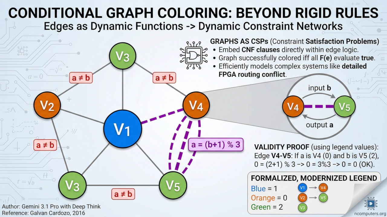
Now, the solution from the previous graph would not be valid for the following graph, where one edge has the function a = (b + 1) % 3. Therefore, it was necessary to change to another solution.
Conditional Coloring Graph Example
A specific edge has a custom mathematical function
The traditional solution is now invalid. A new layout is required to satisfy the specific condition if a=V4 and b=V5: Orange(0) = (Green(2) + 1) % 3.
Optimizing FPGA Routing with Conditional Coloring
Any graph can be modeled with specific functions on each edge, or a global function for all edges. This has proven to be highly useful for modeling detailed connectivity in FPGAs (Field-Programmable Gate Arrays), which have certain strict physical limitations and restrictions in the routing between their internal logic modules.
Naturally, the more specific functions are added to each edge, the more complex the graph becomes. This transforms the routing challenge into a more sophisticated Constraint Satisfaction Problem (CSP). To resolve this efficiently, pairing conditional coloring with advanced heuristic search trees—like the multidimensional R-tree mentioned in the referenced thesis—allows algorithms to instantly pinpoint and recalculate only the conflicting sub-sections of the graph, making routing solutions both fast and extremely accurate.